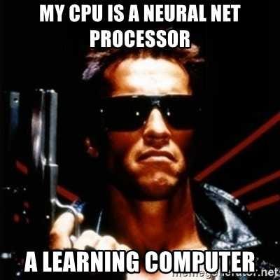
Large Language Models (LLMs) have been the buzz since 2021. One of the most popular ones being ChatGPT, followed by Gemini and then Claude…
The Complete Dummies’ Guide to LLMs #
Large Language Models (LLMs) have been the buzz since 2021. One of the most popular ones being ChatGPT, followed by Gemini and then Claude. But these are just the tip of the iceberg. LLMs have revolutionized natural language processing and artificial intelligence. However, the field is rife with complex terminology that can be daunting for newcomers. This guide aims to demystify key concepts and jargon related to LLMs, making the subject more accessible to a wider audience.

This article is best read with a foundational level of knowledge on machine learning, backpropagation and computational mathematics.
Table of Contents #
- A Brief overview of LLMs and their importance
- Demystifying LLM terminology
- How LLMs learn
- Transformers 101
- You Just Want Attention
- Training and Inference
- Finetuning
- Advanced Finetuning Techniques
- Model Initialization
- Quantization
- A Brief Survey on Quantization Techniques
- Advanced Quantization Techniques
- Inference and Training Arithmetic
- LLM Pollution
- Conclusion: Putting it all together
A Brief Overview of LLMs and their importance #
Language Model Models (LLMs) have gained immense popularity in recent years due to their ability to generate human-like text. These sophisticated algorithms, developed using deep learning techniques, have found a wide range of applications in various fields.
LLMs are essentially very, very deep neural networks (DNNs). For those of you don’t know what a deep (or even a neural network is), check this article out.
DNNs are known for their ability to capture latent (hidden) information, sequences and/or patterns within large data. Deep neural networks are particularly useful in computer vision and language modelling tasks, where a regular statistical algorithm may fail to fit to larger data.
Going back again, a very deep NN with the right architecture to learn latent representations within text data is what basically an LLM does. And this is quite important in the real world, where text-based tasks such as conventional business, conversation and translation require mass automation. LLMs had found their initial footing here.

It has been a few years since LLM has taken over the internet. Now everyone can communicate with their own LLMs through ChatGPT, Gemini, etc.
Now, you can even personalize your own LLM for your needs.

But later on that part ;)
Demystifying LLM Terminology #

You may have heard terms such as agents, few shot learning, finetuning, GPTs, hallucination, RAG, hybrid search, training, inference, blah blah blah. If you haven’t, dont’t fret.
Let’s cover a lot more than few concepts:
0. Foundational Models:
The gods of Generative AI. The Stanford Institute for Human-Centered Artificial Intelligence’s (HAI) Center for Research on Foundation Models (CRFM) coined the term “foundation model” in August 2021 to mean “any model that is trained on broad data (generally using self-supervision at scale) that can be adapted (e.g., fine-tuned) to a wide range of downstream tasks”.
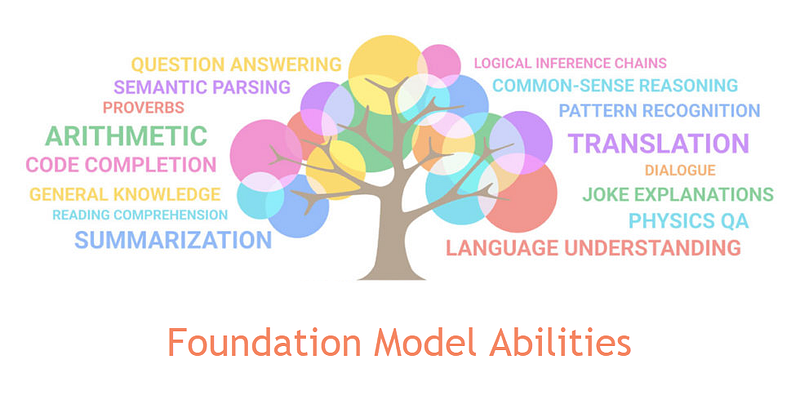
In a nutshell, large foundation models such as Microsoft Florence (Vision), OpenAI’s GPT (coming up), CLIP (image captioning), Diffusion (Image Generation) have been retrained countless times on different data to meet different needs, but their core architecture and learned representation stay more or less the same, making it easier to build newer models from these gods.
1. GPTs:

Abbreviation for ‘Generative Pre-Trained Transformer’. These are a class of LLMs that are built on the transformer architecture, a type of very deep DNN that has been proven to perform remarkably well on long range sequences.
2. Agents:

LLM agents are advanced AI systems designed for creating complex text that needs sequential reasoning. They can think ahead, remember past conversations, and use different tools to adjust their responses based on the situation and style needed. You can deploy a crew of agents specialized for automating a task, for instance, managing your emails, attending your calls while away, digging up research material, etc. CrewAI has a well-developed suite for Agentic AI.
3. Hallucination:
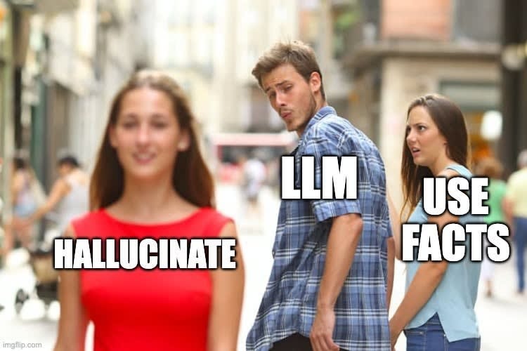
Yes, it’s LLMs making up stuff just like we do when giddy. Hallucinations in LLMs refer to the generation of content that is irrelevant, made-up, or inconsistent with the input data. This problem leads to incorrect information, challenging the trust placed in these models. Wanna try? Go ahead and ask Gemini or ChatGPT something that is partially true and after a couple of prompts, it should start hallucinating ;)
4. Retrieval Augmented Generation (RAG):
One step closer to your personal AI, RAG is an easy and popular way to use your own data by providing it as part of the prompt with which you query the LLM model. The name stands as you would retrieve the relevant data and use it as augmented context for the LLM. Instead of relying solely on knowledge derived from the training data, a RAG workflow pulls relevant information and connects static LLMs with real-time data retrieval.

A RAG workflow consists of the User, the LLM and a Vector Database (VDB). The VDB can be modified and updated however well you want the LLM to refer to ‘your’ factual information. Pinecone, Chroma and Weaviate are renowned cloud-based VDBs for integrating into your RAG workflow.

If you’ve ever encountered the above messages while playing around, it’s because Web-based RAG wasn’t a feature yet. Now almost all LLM giants implement a RAG pipeline with access to the internet to stay up to date.
5. Hybrid Search:
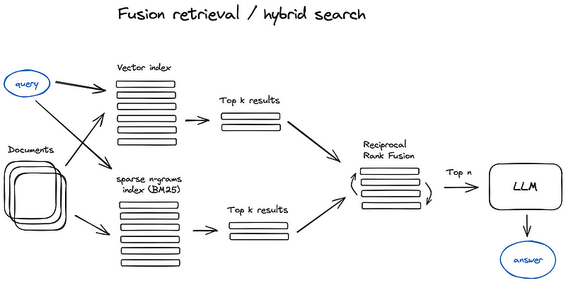
It’s a cross between semantic search and RAG. Dumbing it down, it is a combination of keyword search and neural networks.
A relatively old idea that you could take the best from both worlds — keyword-based old school search — sparse retrieval algorithms like tf-idf or search industry standard BM25 — and modern semantic or vector search and combine it in one retrieval result.
The only trick here is to properly combine the retrieved results with different similarity scores — this problem is usually solved with the help of the Reciprocal Rank Fusion algorithm, reranking the retrieved results for the final output.
Algolia and Cohere are pretty well-known hybrid search engines.
6. Prompt Engineering:

It is the process of crafting, refining, and optimizing the input prompts given to an LLM in order to achieve desired outputs. Prompt engineering plays a crucial role in determining the performance and behavior of models like those based on the GPT architecture.
If you’re a seasoned ChatGPT user, you would be knowing well that it requires a lot more than small talk to get things done. Unofficially, everyone is a prompt engineer!
7. Upstream and Downstream Tasks:
In the world of Large Language Models, we often talk about upstream and downstream tasks. But what do these aquatic-sounding terms actually mean? Let’s dive in!
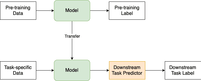
Imagine an LLM as a mighty river of knowledge. Upstream tasks are like the mountain springs and tributaries that feed this river. These are the fundamental tasks that help the model learn general language understanding and generation. Examples include:
- Next word prediction
- Masked language modeling
- Sentence completion
These tasks are the heavy lifters, shaping the riverbed and determining the flow of the AI river.
Downstream tasks are like the various activities you can do once the river is flowing strong. These are specific applications or fine-tuned uses of the pre-trained model. Examples include:
- Sentiment analysis
- Named entity recognition
- Text summarization
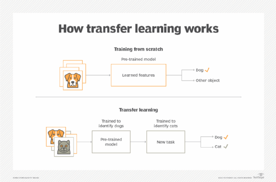
8. Transfer Learning

Training an LLM model is a huge, costly and painful task (I’m gonna give you the gore details later on). Transfer learning popped into the picture when researchers realized you could attain almost the same accuracy, precision and capabilities of the parent model with little to no loss by transferring its knowledge to a smaller daughter model.
YOLO is a family of Computer Vision, Detection and Segmentation models that are initially trained on a huge number of classes and even huger datasets (we’re talking hundreds of gigabytes here). But regular folk may not need the entire model for their usecase. Perhaps you need to just detect a cat or dog for a project, or maybe a new object that is not in the parent model. YOLO has transfer learned its parameters to smaller variants for ease-of-use and deployment.
That’s it for now. We still have a lot more to tour!
How LLMs Learn #
Large Language Models (LLMs) are like digital sponges that have devoured entire libraries. But how exactly do these binary marvels acquire their knowledge? Let’s break it down.
1. The Data Buffet

Imagine a massive, all-you-can-eat buffet of text. LLMs start their journey by ingesting enormous amounts of text data from various sources:
- Books
- Websites
- Articles
- Social media posts
- And pretty much anything else written by humans
2. Pattern Recognition: The Digital Sherlock
As LLMs consume this data, they’re not just memorizing; they’re detecting patterns. They become experts at recognizing:
- How words are typically used together
- Common sentence structures
- Context-dependent meanings
Internally, it’s all just simple matrix multiplication happening billions of times per second, updating each parameter in the network. It’s pretty much modelled after how the brain learns. Hot mess really.
3. The Magic of Neural Networks

Under the hood, LLMs use complex neural networks, typically based on the Transformer architecture. These networks consist of:
- Input layers: Where the text goes in
- Hidden layers: Where the magic happens
- Output layers: Where predictions come out
As the model processes more data, it adjusts the strengths of connections between these layers, fine-tuning its understanding.
4. Training Objectives: The Guessing Game
LLMs often learn through what’s called “unsupervised learning.” A common technique is “masked language modeling,” where:

1. The model is shown a sentence with some words masked out
2. It tries to predict the masked words
3. It checks its guesses against the actual words
4. It adjusts its internal connections based on how well it did
It’s like filling in blanks in a giant, cosmic Mad Libs game!
5. Iteration and Optimization
Learning for an LLM is an iterative process. It goes through the data multiple times (called epochs), each time:
- Making predictions
- Calculating how far off it was (loss function)
- Adjusting its internal parameters to do better next time (backpropagation)

This process continues until the model’s performance stops improving significantly.
6. The Never-Ending Quest
Even after initial training, many LLMs continue to learn through fine-tuning on specific tasks or datasets. It’s like sending a language graduate to a specialized finishing school.

In essence, LLMs learn by consuming vast amounts of text, playing prediction games with themselves, and constantly fine-tuning their understanding based on their successes and failures. It’s a bit like how humans learn language, just at a much, much larger scale and speed!
Transformers 101 #

Transformers are the architectural backbone of modern Large Language Models. Introduced in the 2017 paper “Attention Is All You Need,” they revolutionized natural language processing. Think of Transformers as the secret sauce that makes your AI assistant sound so smart!
The Building Blocks

Imagine Transformers as a high-tech assembly line for processing language. The ingredients are fed in, i.e. structured prompts, and the product is spat out, i.e. structured responses. Here are the key components:
1. Input Embedding
- Converts words into number vectors
- Like translating human language into “machine-speak”
2. Positional Encoding
- Adds information about word order
- Because in “Dog bites man” and “Man bites dog,” order matters!
3. Multi-Head Attention
- The “pay attention” mechanism, something we’ll talk about later
- Allows the model to focus on different parts of the input simultaneously
- Like having multiple readers, each focusing on different aspects of a text
4. Feed-Forward Neural Networks
- Processes the attention output
- Adds depth to the model’s understanding
5. Layer Normalization and Residual Connections
- Keeps the signal from getting too wild
- Helps information flow smoothly through the model
The Transformer Dance: Encoding and Decoding
Transformers typically have two main parts:
1. Encoder: Processes the input
— Like a super-efficient reader, understanding the context
2. Decoder: Generates the output
— Like a talented writer, crafting responses based on the encoder’s understanding
Some models, like BERT, use only the encoder, while others, like GPT, use only the decoder. Full Transformer models use both.
The Secret Sauce: Self-Attention
The real magic of Transformers lies in their self-attention mechanism. Here’s how it works:
1. For each word, create three vectors: Query, Key, and Value
2. Calculate attention scores between the Query and all Keys
3. Use these scores to create a weighted sum of Values
It’s like each word asking, “How relevant are you to me?” to every other word in the sentence.
And we are diving deep into attention in the next section.
You Just Want Attention: Understanding Attention Mechanisms in Transformers #
Why All the Fuss About Attention? #

In the world of Large Language Models, attention isn’t just a catchy Puth song — it’s the secret sauce that makes these models so powerful. Attention mechanisms allow models to focus on relevant parts of the input when producing output. It’s like having a super-smart reader who knows exactly which parts of a text are important for answering a question.
Brief history of Attention #
Memory is attention through time. ~ Alex Graves 2020
The attention mechanism emerged naturally from problems that deal with time-varying data (sequences). So, since we are dealing with “sequences”, let’s formulate the problem in terms of machine learning first. Attention became popular in the general task of dealing with sequences.
Before attention and transformers, Sequence to Sequence (Seq2Seq) worked pretty much like this:
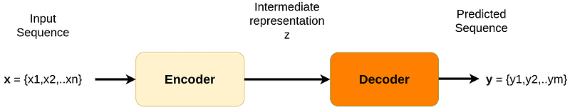
The elements of the sequence x1, x2, y1, y2, etc. are usually called tokens. They can be literally anything. For instance, text representations, pixels, or even images in the case of videos.
OK. So why do we use such models?
The goal is to transform an input sequence (source) to a new one (target).
The two sequences can be of the same or arbitrary length.
In case you are wondering, recurrent neural networks (RNNs) dominated this category of tasks. The reason is simple: we liked to treat sequences sequentially. Sounds obvious and optimal? Transformers proved us it’s not!
Remember about our encoder and decoder friends? #
The encoder and decoder are nothing more than stacked RNN layers, such as LSTM’s. The encoder processes the input and produces one compact representation, called z, from all the input timesteps. It can be regarded as a compressed format of the input.

On the other hand, the decoder receives the context vector z and generates the output sequence. The most common application of Seq2seq is language translation. We can think of the input sequence as the representation of a sentence in English and the output as the same sentence in French.

In fact, RNN-based architectures used to work very well especially with LSTM and GRU components. It was also a lot softer in terms of time and space complexity: being linearly complex.
The problem? It only worked effectively for small sequences (<20 timesteps). A ton of issues arose with vanishing and exploding gradients, non-parallel computation (linear complexity) and required lots of training steps (epochs).
Attention was born in order to address these two things on the Seq2seq model. But how?
The core idea is that the context vector z should have access to all parts of the input sequence instead of just the last one.
In other words, we need to form a direct connection with each timestamp.
How Attention Works #
Let’s start with why attention is getting all the hype. It’s not just a trendy buzzword — it’s the result of years of research compounding successful results. But like any groundbreaking technology, it comes with its trade-offs.
Attention is a memory guzzler. With its quadratic space and time complexity, it’s like a luxury car that demands premium fuel. If Recurrent Neural Networks (RNNs) could perform just as well with their linear complexity, we might not be so obsessed with attention.
Attention brings something revolutionary to the table. When you feed an input to a model with attention:
- It selectively focuses on the most important parts of the input
- It studies these parts contextually
- It can easily connect distant parts of the input
Let’s compare: #
1. RNNs (The Old Guard):
- Process information sequentially
- Pay attention to everything equally
- Struggle with long-range dependencies
- Like trying to remember the beginning of a long story while still reading the end
2. Attention Mechanisms (The New Sheriff):
- Can jump back and forth between different parts of the input
- Selectively focus on what’s important
- Excel at understanding long-range context
- Like having a perfect memory of the entire story while reading any part
Let me break this down with the help of an example:

A literal translation of the German sentence to English sounds weird, as we’re mapping each German word directly to its literal English counterpart without considering contextual semantics. The targeted English translation however requires a broad sense of the grammar, syntax and semantics that the German and English language carry across each other. Attention captures this inherent and latent grammar semantic by learning to attend to the most common words. In the example, notice that the words ‘mir’, ‘helfen’, ‘Satz’, etc. ie, the ones that cross positions during translation are the mappings that our model pays more attention to.
Let me simplify this further with a visualization:

In this visualization, notice how the brightest lines connect the words that need special attention for correct translation. Words that stay in roughly the same position have weaker attention connections. Some words attend to multiple other words, showing how the context is built.
All in all, the attention model learns to pay more attention to:
- Words that typically change position during translation
- Key contextual markers that signal how the sentence structure should change
- Words that have multiple possible translations, choosing the right one based on context
Alright, but what am I supposed to do with this attention information? Obviously train the model, but how? And what is attention generating that I can use to train the model with? Remember our short discussion on query, key and value vectors?

The way attention is calculated is a bit complex. Let’s dissect the Encoder part of the LLM to understand how attention works:
Encoder #
Step 1
For each input sentence fed into the encoder, we first encode it (positional encoding, remember?) and then embed it into a vector space. The input embeddings are then multiplied with 3 matrices:
- Query weight matrix (Wq) x Input = Query Matrix (Q)
- Key weight matrix (Wk) x Input = Key Matrix (K)
- Value weight matrix (Wv) x Input = Value Matrix (V)
And logically, what do these resultant matrices signify?
- Query is like the question you have in mind (“Who knows about AI?”)
- Key is like the name tags people wear (“AI Engineer”, “Data Scientist”)
- Value is the actual knowledge each person has
Step 2
The attention formula allows us to calculate the attention score:
Attention(Q, K, V) = softmax((Q * K^T) / √d_k) * V
Query and key undergo a dot product matrix multiplication to produce a score matrix. The score matrix contains the “tensor or weights” distributed to each word as per its influence on input.
The weighted attention matrix does a cross-multiplication with the “value” vector to produce an output sequence. The output values indicate the placement of subjects and verbs, the flow of logic, and output arrangements.
However, multiplying matrices within a neural network may cause exploding gradients and residual values. To stabilize the matrix, it’s divided by the square root of the dimension of the queries and keys.
Step 3
The softmax layer receives the attention scores and compresses them between values 0 to 1. This gives the machine learning model a more focused representation of where each word stands in the input text sequence.
In the softmax layer, the higher scores are elevated, and the lower scores get depressed. The attention scores [Q*K] are multiplied with the value vector [V] to produce an output vector for each word.
This is followed by residual and layer normalization, which in layman terms translates to eliminating outliers and gradient stabilization (just security checks).

Step 4
The feedforward layer receives the output vectors with embedded output values. It contains a series of neurons that take in the output and then process and translate it. As soon as the input is received, the neural network triggers the ReLU activation function to eliminate the “vanishing gradients” problem from the input.
This gives the output a richer representation and increases the network’s predictive power. Once the output matrix is created, the encoder layer passes the information to the decoder layer.
This is the attention mechanism boiling within the encoder. But what happens in the decoder?
Decoder #
The decoder architecture contains the same number of sublayer operations as the encoder, with a slight difference in the attention mechanism. Decoders are autoregressive, which means it only looks at previous word tokens and previous output to generate the next word.
Let’s look at the steps a decoder goes through.
- Positional embeddings: The decoder takes the input generated by the encoder and previous output tokens and converts them into abstract numeric representations. However, this time, it only converts words until time series t -1, with t being the current word.
- Masked multi-head attention 1: To further prevent decoders from processing future tokens, it undergoes the first layer of masked attention. In this layer, attention scores for decoders are calculated and multiplied by a masked matrix that contains a value between 0 and infinity.
- Softmax layer: After multiplication, the output gets passed on to the softmax layer, which downsizes it and stabilizes the numbers. All the parts of the matrix that belonged to future words are zeroed out. The masked matrix is structured in such a way that negative infinities get multiplied only by future tokens, which are nullified by the softmax layer.
- Masked multi-head attention 2: In the second masked self-attention layer, the value and keys of the encoder output are compared with the decoder output query to get the best output path.
- Feedforward neural network: Between these self-attention layers, a residual feedforward network exists to identify missing gradients, eliminate residue, and train the neural network on the data.
- Linear classifier: The last linear classifier layer predicts the most likely next word. This occurs till the entire response is complete.
Training and Inference #
Think of training and inference as two distinct phases in an LLM’s life:
- Training: The education phase — expensive, time-consuming, but essential
- Inference: The working phase — where the model applies what it learned

What Happens During Training? #
- Data Ingestion: The model processes massive amounts of text data, typically hundreds of gigabytes to petabytes. Example: GPT-3 trained on 45TB of compressed text!
- Parameter Updates: The model adjusts billions of parameters and uses backpropagation to minimize loss function as well as techniques for gradient descent optimization.
- Validation: Regular testing on held-out data and ensures model isn’t just memorizing (overfitting)
Training Requirements:
- Time: Days to months
- Hardware: Multiple high-end GPUs/TPUs
- Memory: Hundreds of GB of VRAM
- Cost: Can run into millions of dollars

What Happens During Inference?
- Input Processing: Tokenization of user input and converting tokens to model’s input format.
- Forward Pass: Only uses the forward path through the network without parameter updates. Much faster than training.
- Output Generation: Typically uses beam search, reranking and sampling methods (more on this in RAG).
Inference Requirements:
- Time: Milliseconds to seconds
- Hardware: Can run on consumer GPUs or even CPUs
- Memory: Can be optimized (quantization, upcoming)
- Cost: Fraction of training costs
+------------+---------------------------+----------------------------+
|   Aspect   |         Training          |         Inference          |
+------------+---------------------------+----------------------------+
| Direction  | Forward + Backward        | Forward only               |
| Memory     | High (gradients)          | Lower (no gradients)       |
| Speed      | Slow (parameter updating) | Faster (fixed parameters)  |
| Batch Size | Large (for stability)     | Small (for responsiveness) |
+------------+---------------------------+----------------------------+
PS: When you initiate a conversation with ChatGPT (termed ‘initialization’), the servers at OpenAI are essentially loading the entire GPT model onto their hardware for inference. Since ChatGPT is quite large (in the range of hundreds of billions of parameters), they require large-scale compute infrastructure (distributed across multiple GPUs) just to hold a single conversation with a user. Talk about free plans!
However, whenever OpenAI releases a new model, it has a long history of training on much larger accelerated hardware. Thousands of GPUs, efficient attention mechanisms and better training data. This is where most of the funding, grants and a large portion of collected revenue go into.
Fine-tuning #
Throughout the article, I have been throwing around this term. But what exactly is fine-tuning?
Imagine you have a guitar. When it comes out of the factory, it’s built to play music (like a pre-trained model), but it needs tuning for optimal performance. Just as there are different ways to tune a guitar, there are various techniques to fine-tune a language model.

I will be moving forward with this guitar analogy to keep things simple.
What is fine-tuning? #
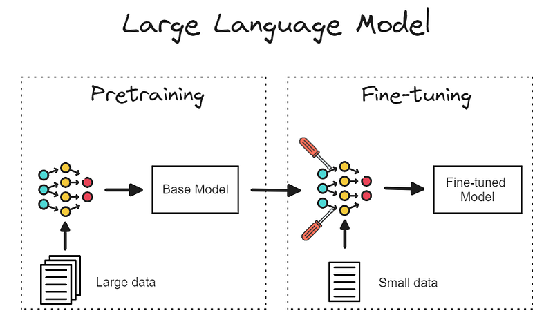
Fine-tuning is the process of taking a pre-trained model and adapting it to a specific task or domain. It’s like adjusting your guitar strings to play in a different key.
Why fine-tune? #
Just like when a guitar is manufactured to play any sort of music, they can be tuned to perform better on jazz, rock or blues. This requires careful tuning of the strings and pegs by the guitarist.
In the same space, LLMs understand language structure very well and are poised to respond to any text input. Just as you might tune a guitar differently, LLM behavior can be adjusted for sentiment analysis, translation, etc. Fine-tuning is easier than building and training a new model from scratch. Just like choosing to tune a guitar rather than building a new one entirely.
For example, did you know that GPT-3.5 and GPT-4 are LLMs fine-tuned from a larger foundational GPT? LLaMa, the open-source LLM released by Meta, has been fine-tuned for millions of tasks, ranging from customer service to personal chatbots to even for-profit applications.
Let’s look into the two approaches to fine-tuning:
Standard Tuning: Full Fine-tuning #
Like tuning all strings on a guitar (E, A, D, G, B, E), full fine-tuning adjusts all layers of the model. In terms of data, this task requires a huge dataset relevant to the task it has to be specialized on. But this requires large computational resources and might not be a suitable option in the long run, owing to model adaptations.
Drop D Tuning: Partial Fine-tuning #
Like lowering just the low E string to D, partial fine-tuning adjusts only some layers. The layers that are not involved in training are ‘frozen’ and the rest are retrained. This preserves lower-level features that the original model has learned. A better example: if you’re decent at speaking American English, it’s not that hard to catch up on British English.
Advanced Fine-tuning Techniques #
Just as a guitarist might adjust their instrument for different musical styles, we can fine-tune our language models in various ways. Let’s explore advanced fine-tuning techniques through the lens of guitar tuning!
Pruning: Trimming the Excess #

Pruning is a technique that involves removing unnecessary connections or parameters from a neural network. Basically, pruning removes the weights that don’t really matter, making the model smaller and easier to handle. This results in faster speeds and less memory usage — pretty neat, right?
Imagine a guitarist tuning their guitar before a performance. The guitar has six strings, but not every string is needed for every song. Some strings might even produce unnecessary noise or overpower the melody. To make the sound cleaner and more precise, the guitarist decides to adjust or mute certain strings while playing a specific piece. Infact, Keith Richards, songwriter and guitarist for the band ‘Rolling Stones’, used a restricted string setup with only five strings instead of six!
Transfer Learning #
Transfer learning is like teaching a general musician to specialize in guitar. They already know finger placement, reading music, and rhythm; they just need to adapt these skills to a new style.
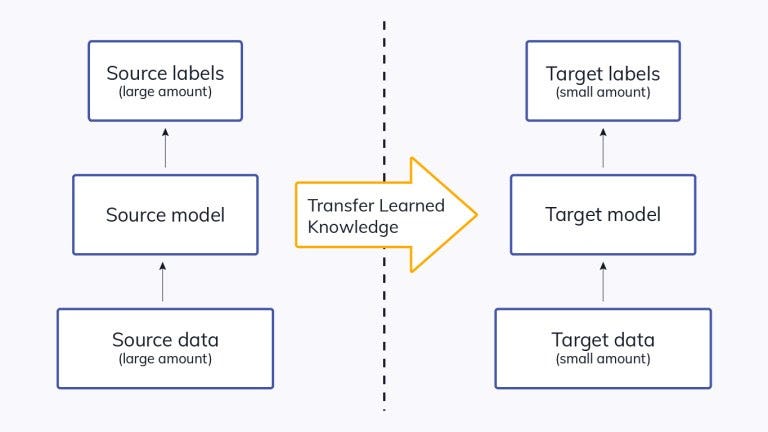
Similarly, in machine learning and deep learning, transfer learning involves taking a model that has already been trained on a general task and fine-tuning it for a new, more specific task. The model has already learned useful features and patterns from a large, broad dataset (like the musician’s general skills). Instead of training a new model from the ground up, we just tweak the existing model to adapt to the new problem, making the process much faster and more efficient.
This way, just as the musician quickly becomes proficient at guitar, the model quickly learns to perform well on the specialized task without needing extensive retraining.
Distillation: Knowledge Transfer for Efficiency #
Think of distillation like a guitarist teaching a student how to play complex songs. The guitarist (the larger model) knows all the advanced techniques, chords, and intricate details of the music. However, the student (the smaller model) doesn’t need to learn every single detail to perform the song well. Instead, the guitarist simplifies the lessons, focusing on the essential techniques and patterns that still capture the essence of the performance.

You’ve got it now!
Distillation involves training a smaller, more compact model to mimic the behavior of a larger, more complex model. By transferring knowledge from the larger model, distillation enables the creation of highly efficient models without sacrificing performance.
This technique has been particularly effective in scenarios where computational resources are limited, such as deploying models on edge devices, smartphones, tablets, etc. A large language model can be distilled into a smaller model that retains most of the original model’s performance while being more lightweight and faster to execute.
Prefix Tuning #
Prefix tuning adapts pre-trained language models to specific tasks without modifying the original model’s weights.
Prefix tuning draws inspiration from the concept of prompting, where task instructions and examples are prepended to the input to steer the LM’s generation. However, instead of using discrete tokens, prefix tuning uses a continuous prefix vector.
Prefix-tuning involves prepending a sequence of continuous task-specific vectors, called a prefix, to the input of the LM.
The Transformer can attend to these prefix vectors as if they were a sequence of “virtual tokens”. Unlike prompting, the prefix vectors do not correspond to real tokens but are learned during training.
LoRA: Low Rank Adaptation #
Now imagine adding a small device to your guitar that, when activated, changes how certain chords sound:
- The guitar’s main structure remains unchanged
- The device affects only specific combinations of strings
- You can easily swap devices for different effects

LoRA adds small, trainable rank decomposition matrices. These matrices are like “adapters” for the model and modifies the model’s behavior without changing most weights. So instead of retraining a subset of the model, we retrain these decomposable matrices, saving us a ton of time and compute. This make LoRA much more memory efficient than full fine-tuning.
QLoRA: Quantized LoRA #
Like practicing an electric guitar without an amp:
- The guitar’s full potential is compressed
- You can still learn and practice effectively
- When you plug in, you get the full sound
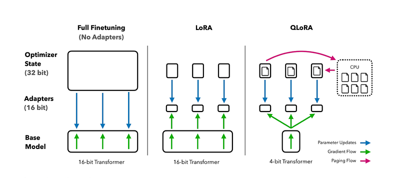
QLoRA takes LoRA a step further by also quantizing the weights of the LoRA adapters (smaller matrices) to lower precision (e.g., 4-bit or 8-bit instead of 16-bit). This further reduces the memory footprint and storage requirements. QLoRA is even more memory efficient than LoRA, making it ideal for resource-constrained environments.
Choosing between LoRA and QLoRA: #
The best choice between LoRA and QLoRA depends on your specific needs:
- If memory footprint is the primary concern: QLoRA is the better choice due to its even greater memory efficiency.
- If fine-tuning speed is crucial: LoRA may be preferable due to its slightly faster training times.
- If both memory and speed are important: QLoRA offers a good balance between both.
There’s a lot more variants of LoRA such as ReLoRA, SLoRA, GaLoRA, etc. But discussing them is out of the scope of this article as they require other your understanding of a few other foundational theories. If you do want to check them out, here is a good article that explain each technique in precise detail.
Prompt Engineering #
The process of crafting, refining, and optimizing the input prompts given to an LLM in order to achieve desired outputs. Prompt engineering plays a crucial role in determining the performance and behavior of models like those based on the GPT architecture.
Given the vast knowledge and diverse potential responses a model can generate, the way a question or instruction is phrased can lead to significantly different results. Some specific techniques in prompt engineering include:
- Rephrasing: Sometimes, rewording a prompt can lead to better results. For instance, instead of asking “What is the capital of France?” one might ask, “Can you name the city that serves as the capital of France?”
- Specifying Format: For tasks where the format of the answer matters, you can specify it in the prompt. For example, “Provide an answer in bullet points” or “Write a three-sentence summary.”
- Leading Information: Including additional context or leading information can help in narrowing down the desired response. E.g., “Considering the economic implications, explain the impact of inflation.”
Zero-Shot, One-Shot and Few-Shot Learning #
These are techniques that do not strictly fall under fine-tuning, but rather more into Prompt Engineering. Here, the model adapts to new tasks by providing it with no (zero-shot), one (one-shot) or multiple (few-shot) data samples of the intended tasks.
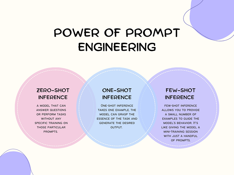
How Few-Shot Learning Works #
- Provides the model with a few examples
- Model recognizes patterns in these examples
- Applies these patterns to new, similar tasks
This typically works on large parameter models like the GPT series or the Llama 3 70B onwards.
Reinforcement Learning through Human Feedback (RLHF) #
If you’ve used ChatGPT quite enough, you may have noticed that you do get occasionally prompted on how you would rate it’s response. Or whether it requires an improvement. Or to make a choice on the better of the two responses.
These are all inputs to an RLHF framework that will be involved in iterative fine-tuning of the base GPT later on. It’s similar to a club guitarist who plays different variations of a song, gauges the audience’s reaction, and adjusts their playing based on feedback.
How RLHF Actually Works #

- Initial Training: Model learns basic capabilities
- Reward Modeling: Human feedback is collected. A reward model is trained to predict human preferences
- Reinforcement Learning: Model is further trained using the reward model. Behaviors that align with human preferences are reinforced
Components of RLHF #
- Base Model: The initial pre-trained model
- Reward Model: Learns to predict human preferences
- Policy Model: The model being fine-tuned
- Human Feedback: Crucial for guidance
Model Initialization: Hot, Cold or Frozen Start? #
The Thermal Spectrum of Starting Models #
When it comes to initializing Large Language Models, we have three main approaches:
- Cold Start: Starting from scratch. The model weights are initialized randomly, and the model is trained from ground zero with no prior knowledge utilized. Cold start is used where novel architectures have to be trained, and/or there is no existing pre-trained architecture to support the new one. Eg: GPT-4 API usage
- Warm/Hot Start: Beginning with pre-trained weights from an existing model, we fine-tune all layers for a domain-specific task. This is also interchangeably called transfer learning. This initialization method is useful when the model behavior has to be adapted significantly on task-specific data. Eg: BERT Fine-tuning
- Frozen Start: Using a pre-trained model with fixed parameters, we freeze almost all the model’s parameters and only train new task-specific layers. This is useful when you have limited VRAM or compute (sad GTX noises) and a very small dataset. Eg: Opensource LLM fine-tuning.
Quantization #

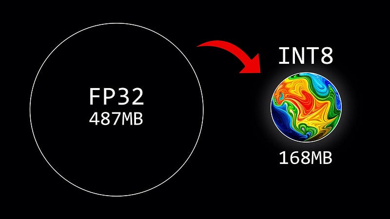
Quantization aka Compression, especially in AI models and deep learning models, typically refers to converting the model’s parameters, such as weights and biases, from floating-point numbers to integers with lower bit widths, for example, from 32-bit floating-point to 8-bit integers. In simple terms, quantization is like simplifying a detailed book written with high-level vocabulary into a concise summary or a children’s version of the story. This summary or children’s version takes up less space and is easier to communicate, but it may lose some of the details present in the original book.
Why Quantization #
The purpose of quantization mainly includes the following points:
1. Reduced Storage Requirements: Quantized models have significantly smaller sizes, making them easier to deploy on devices with limited storage resources, such as mobile devices or embedded systems.
2. Accelerated Computation: Integer operations are generally faster than floating-point operations, especially on devices without dedicated floating-point hardware support.
3. Reduced Power Consumption: On certain hardware, integer operations consume less energy.
There is often some loss of precision (granularity) when reducing the number of bits to represent the original parameters.
To illustrate this effect, we can take any image and use only 8 colors to represent it:
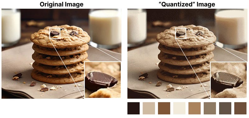
Notice how the zoomed-in part seems more “grainy” than the original since we can use fewer colors to represent it.
The main goal of quantization is to reduce the number of bits (colors) needed to represent the original parameters while preserving the precision of the original parameters as best as possible.
However, quantization has a drawback: it can lead to a reduction in model accuracy. This is because you are representing the original floating-point numbers with lower precision, which may result in some loss of information, meaning the model’s capabilities may decrease.
To balance this accuracy loss, researchers have developed various quantization strategies and techniques, which we’ll be seeing soon.
A Brief Survey on Quantization Techniques #
Two primary machine and deep learning model quantization modes exist — PTQ and QAT. Let’s understand them both.
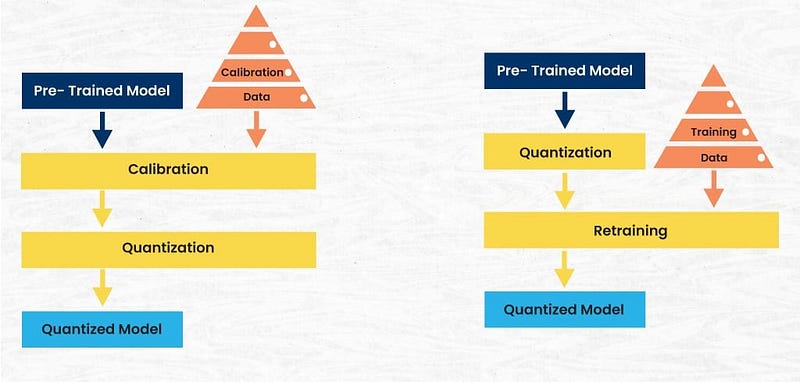
Quantization Aware Training (QAT) #
- We start QAT with a pre-trained model or a PTQ model. We fine tune this model using QAT. The aim here is to recover the accuracy loss that happened due to PTQ in case we took a PTQ model.
- The basic idea of QAT is to quantize input into lower precision depending on the weight precision of that layer. QAT also takes care of converting the output of multiplication of weights and inputs back to higher precision in case the next layer demands so. This process of converting input to lower precision and then converting output of weights and inputs back to higher precision is also called as “FakeQuant Node Insertion”. The quantization is called Fake as it quantizes and then dequantizes as well converting to the base operation.
Post-Training Quantization #
- Post-Training Quantization (PTQ) is a technique that allows us to quantize a pre-trained model after the training process is complete, without requiring any further training or fine-tuning. The goal of PTQ is to reduce the size and computational requirements of the model by converting its weights and activations to lower precision, typically 8-bit integers, while preserving as much accuracy as possible.
- In PTQ, the model is first evaluated with a calibration dataset to collect statistics, which are then used to determine the optimal quantization parameters (scale and zero-point) for each layer. Unlike Quantization Aware Training (QAT), there is no need to modify the training process itself. PTQ is often faster to implement than QAT since it does not require retraining.
- During inference, both the weights and activations are quantized to lower precision. However, PTQ does not simulate quantization in the training process, which can lead to some loss in accuracy, especially for models with highly sensitive layers. The method is more straightforward compared to QAT but may struggle to recover accuracy loss without additional fine-tuning, as it doesn’t learn to adjust to the quantization-induced errors.
Advanced Quantization Techniques #
FP16/INT8/INT4 #
Popularly, if a model’s name doesn’t have specific identifiers like Llama-2–7b or chatglm2–6b, it generally indicates that these models are in full precision (FP32), although some may also be in half-precision (FP16). However, if the model’s name includes terms like fp16, int8, int4, such as Llama-2–7B-fp16, chatglm-6b-int8, or chatglm2–6b-int4, it suggests that these models have undergone quantization, with fp16, int8, or int4 denoting the level of quantization precision.
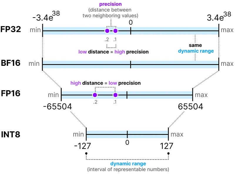
The quantization precision ranges from high to low as follows: fp16 > int8 > int4. Lower quantization precision results in smaller model sizes and reduced GPU memory requirements. Still, it can also lead to decreased model performance.
GPTQ #
GPTQ stands for Generalized Post Training Quantization. This means once you have your pre trained LLM, you simply convert the model parameters into lower precision.
GPTQ is preferred for GPU’s & not CPU’s. My poor RTX 3050😅
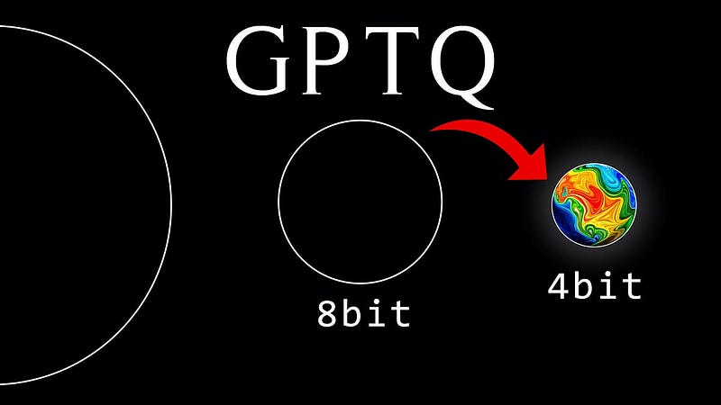
GPTQ is a model quantization method that allows language models to be quantized to precision levels like INT8, INT4, INT3, or even INT2 without significant performance loss. If you come across model names on HuggingFace with “GPTQ” in their names, such as Llama-2–13B-chat-GPTQ, it means these models have undergone GPTQ quantization. For example, consider Llama-2–13B-chat, the full-precision version of this model has a size of 26 GB, but after quantization using GPTQ to INT4 precision, the model’s size reduces to 7.26 GB.
GGML | GGUF #
On HuggingFace, if you come across model names with “GGML,” such as Llama-2–13B-chat-GGML, it indicates that these models have undergone GGML quantization. GGML stands for Generative Graphical Models.
Some GGML model names not only include “GGML” but also have suffixes like “q4,” “q4_0,” “q5,” and so on, such as Llama-2–7b-ggml-q4. In this context, “q4” refers to the GGML quantization method. Q-series quantization methods are a whole other ballgame but there’s a beautiful Reddit thread on this, should you be curious.
GPT-Generated Unified Format aka GGUF is the new version of GGML. GGUF is specially designed to store inference models and adds more data about the model so it’s easier to support multiple older and newer architectures.
GPTQ vs GGML #
GPTQ and GGML are currently the two primary methods for model quantization, but what are the differences between them? And which quantization method should you choose?
Here are some key similarities and differences between the two:
- GPTQ runs faster on GPUs, while GGML runs faster on CPUs.
- Models quantized with GGML tend to be slightly larger than those quantized with GPTQ at the same precision level, but their inference performance is generally comparable.
- Both GPTQ and GGML can be used to quantize Transformer models available on HuggingFace.
Therefore, if your model runs on a GPU, it’s advisable to use GPTQ for quantization. If your model runs on a CPU, GGML is a recommended choice for quantization.
AWQ #
It stands for Activation-aware Weight Quantization
- This is meant for GPU or CPU.
- In this method, we do not quantize all weights; instead, we quantize weights that are not important for our model to retain it’s validity.
- First, the model’s activations are analyzed to determine which weights have the most significant impact on the output. Weights with minimal impact on the activations are quantized more aggressively, while those crucial to model performance are left in higher precision. This selective process minimizes the loss of accuracy commonly seen in uniform quantization methods while reducing the computational and memory demands, allowing the model to run efficiently on GPUs and CPUs.
Inference and Training Arithmetic #

Inference and training arithmetic is essential knowledge for every AIOps engineer and even non-experts. It involves straightforward math and computing resource allocation. I find this topic particularly fascinating because, although there are a limited number of factors involved, they can be creatively combined in countless ways to generate various budget strategies when planning to train an AI model.
This section is a dumbed down explanation of a larger, more detailed reddit thread on Transformers. I’ll distill the basics here into mathematical equations that can be applied on a practical scale.
KV cache #
Yeah that’s our Key (K) and Value (V) vectors in attention. During inference, the transformer performs self-attention, which requires the kv values for each item currently in the sequence (whether it was prompt/context or a generated token). These vectors are provided a matrix known as the kv cache.
The purpose of this is to avoid recalculations of those vectors every time we process a token. With the computed k,v values, we can save quite a bit of computation at the cost of some storage. Per token, the number of bytes we store is:
2 × 2 × nlayers × nheads × dhead
The first factor of 2 is to account for the two vectors, kk and vv. We store that per each layer, and each of those values is a nheads × dhead matrix. Then multiply by 2 again for the number of bytes (we’ll assume 16-bit format).
The flops (floating points operations per second) to compute k and v for all our layers is:
2 × 2 × nlayers × dmodel^2
How many flops in a matmul?
The computation for a matrix-vector multiplication is 2mn, where m × n is the dimension of the matrix and n is the vector. A matrix-matrix is 2mnp, here m × n and n × p are the two matrices.
This means for a 52B parameter model (taking Anthropic’s, where dmodel=8192 and nlayers=64). The flops are
2 × 2 × 64 × 8192^2 = 17,179,869,184 flops
Say we have an A100 GPU, which does 3.12^12 flops per second and 1.5^12 bytes per second of memory bandwidth. The following are numbers for just the kv weights and computations.
memory = 2 × 2 × nlayers × dmodel^2 ÷ 1.5^12
compute = 2 × 2 × nlayers × dmodel^2 ÷ 312^12
Flops vs Memory Boundedness
Flops vs memory boundedness is something we deal with a lot for transformer inference, but also in deep learning optimisation in general. To do the computations we do, we need to load weights which costs memory bandwidth. We assume (correctly, this has been very well optimised) that we can start the computations while we load the weights. Flop bound would then mean that there is time when nothing is being passed through memory, and memory bound would mean that no floperations are occuring. Nvidia uses the term math bandwidth which I find really cute. Technically, this delineation exist per kernel but can be abstracted to exist for groups of operations.
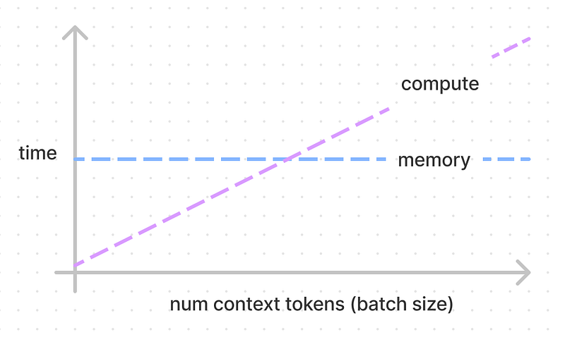
None of the model architecture matters anymore — we get a distinct ratio here of 208 given this hardware specification. This means that if we’re going to compute kv for one token, it’ll take the same amount of time to compute for up to 208 tokens! Anything below, we’re memory bandwidth bound. Above, flops bound. If we used the rest of our weights to do a full forwards pass (run the rest of the transformer) on our context, it’s also 208.
For a 52B model full forwards pass, that’s 12 × 2 × nlayers × dmodel × 2 / 1.5^12 ≈ 69 milliseconds for up to 208 tokens (in practice, we’d use four GPUs in parallel so it would actually be ~17 milliseconds, more in following sections). If we had 416 (double) tokens in the context, then it would take twice as long, and 312 tokens would take 1.5 times as long.
Sounds pretty fast right? Yep, that’s the AI horsepower of GPU💪🏻
Capacity #
We have a solid idea of the two things we store in our GPUs — kv cache and weights. GPU capacity does come into play for transformer inferencing performance, and we have all the understanding we need to evaluate that now!
Nvidia A100 GPUs (which are generally speaking, the best bang for the buck GPUs we can get for inference) have a standard of 40GB of capacity. There are ones with 80GB and higher memory bandwidth (2^12 instead of 1.5^12), but you can deal with different versions with these equations later on.
Given the parameter count, we can multiply by two (assuming 16-bit precision) to get bytes. So, to calculate the size of the weights for a 52B model:
52^12 × 2 = 104^12 bytes ≈ 104GB
Oh no! This doesn’t fit in one GPU! We’d need at least three GPUs just to have all the weights loaded in (will discuss how to do that sharding later). That leaves us 120 − 104 = 16GB left for our kv cache. Is that enough? Back to our equation for kv cache memory per token, again with a 52B model;
2 × nlayers × nheads × dhead × 2 × 4 × nlayers × nheads × dhead = 4 × 64 × 8192 = 2,097,152 bytes ≈ 0.002GB
And then we’d do 16/0.002 ≈ 8000 tokens can fit into our kv cache with this GPU set up. For four GPUs, we’d get 4 × 16/0.002 ≈ 32000 tokens.
Alright, here’s the punchline: #
So, training and inference with transformers boils down to a game of “Flops vs Memory Juggling.” The KV cache is like the secret weapon you stash under your desk — saves you time but takes up space. You’re swapping storage for speed, and GPUs are your best friends in this crazy balancing act.
For any monster model, it’s a lot like trying to cram an elephant into a Mini Cooper — just doesn’t fit! You’re going to need a couple more cars (GPUs) to carry all the weight. You can also simulate the same for the Llama 70B models, or even the larger GPT models (I dare you go read their whitepaper), as long as you have the variables dialled down.
TL;DR: Transformers = doing a lot of math really fast, GPUs are the gym. Jst do your research on Nvidia GPU specs and you’re spot on.
LLM Pollution #
As we navigate through 2024, the AI landscape is experiencing what many experts call “LLM pollution” — an overwhelming proliferation of language models that often contribute more to noise than progress. This phenomenon has only intensified since 2023, with new models being released almost weekly, yet only a fraction finding meaningful applications or user adoption.
The best example for this is Meta’s LlaMa family of models. Since it’s first open-source release with LlaMa in February 2023, many individuals, organizations and communities have retrained, finetuned, quantized and released thousands if not millions of variants of these models for domain-specific usecases. The problem here is there really isn’t proper zero-to-one innovation carrying forward research in AI on improving accuracy, fidelity and reasoning capabilities of LLMs.
As we move forward, the measure of success will be not how many models we can create, but how effectively we can deploy them to solve real-world problems.
Conclusion: Putting It All Together #

Throughout this comprehensive guide, we’ve journeyed through the landscape of Large Language Models, covering essential concepts from the ground up. We explored the foundational transformer architecture, delved into attention mechanisms, and understood the critical distinction between training and inference. We examined various fine-tuning techniques like LoRA and QLoRA, investigated quantization methods from basic INT8 to advanced approaches like GPTQ and GGML, and even tackled the mathematics behind inference arithmetic and KV cache calculations. Along the way, we also addressed practical concerns like model initialization strategies and the challenge of LLM pollution in today’s AI landscape.
Until next time then! Thank you for taking your time reading through the article🤗
By Aloshdenny on October 3, 2024.
Exported from Medium on February 2, 2026.